Having ensured that we have successfully carried out our survey, our research hypotheses were formulated correctly; our sampling was scientifically designed, our survey instruments were constructed correctly, tested and validated and finally, the data were correctly entered onto the computer, our next task is to plan for analyzing the data.
Data analysis is particularly necessary for testing hypotheses or otherwise answers our research questions and to further our overall goal of understanding social phenomena.
Our data may be interpreted and presented in entirely verbal terms, particularly in observational studies, and document studies.
However, when we are dealing with quantitative data, we prefer to employ statistical techniques to analyze our data. Our goal in statistical analysis can be achieved through the process of description, explanation, and prediction.
Of the three tasks, descriptive analysis refers to the transformation of raw data into a form that will make it easy to understand and interpret. Describing responses or observations is typically the first form of analysis.
Descriptive analysis is simply attempted to telling what the data “look like,” for example, how many cases were analyzed, what the range of score was, what was the mean score, how the individual scores differ from each other, and so forth.
This is often conducted for one variable at a time, for which it is qualified as univariate analysis.
Explanation and predictions are generally more complicated than the description and require more comprehension as well as more interpretation.
Explanatory statistical analysis can take several forms but generally consists of the analysis of the relationship between two or more variables.
This is accomplished usually through varieties of statistical techniques: Test of significance, correlation analysis, regression analysis, and the like.

The following section will provide a brief overview of the methods of data analysis about;
- Univariate,
- Bivariate,
- Yri-variate, and
- Multivariate Analysis.
Univariate Analysis
The first step in seeing what your data look like is to examine each variable separately. This can be accomplished by getting the distribution of each variable one by one.
Such single-variable analysis is called univariate analysis, that is, analysis based on one variable. The simplest form of single-variable analysis is to count the number of cases in each category.
The resulting count is called a frequency distribution. We can form frequency distributions of such single variables as religion (which is measured on a nominal scale), level of education (ordinal scale), temperature (interval scale) and age (ratio scale)
A frequency distribution is, however, not usually very interesting and informative without additional statistical manipulations.
Several statistical measures can be obtained from a frequency distribution. Still, the precise nature of the permissible measures will depend on the type of a variable or more accurately on the level of measurement.
The commonly used levels of measurement are nominal, ordinal, and interval, which we have discussed earlier. The accompanying table shows the level of education of a group of women as obtained in the 1993-94 BDH Survey.

The education level shown in column 1 is the only variable measured on an ordinal scale. The distribution is a univariate one.
The second and third columns represent the absolute and percentage frequencies, respectively. The frequencies are absolute numbers and do not lend themselves for meaningful interpretation unless they are standardized for size. This is more so when two or more distributions are to be compared.
Forming proportions or percentages, this problem can be removed. Percentages serve two purposes in data analysis. They simplify by reducing all numbers to a range from 0 to 100.
Second, they translate the data into standard form, with a base of 100, for relative comparison.
Caution must, however, be exercised in using percentages. Note that all percentage values must add to 100 (unless multiple responses are there). And percentage values cannot be averaged ordinarily.
Note that the variable ‘education level’ is a variable measured on an ordinal scale, for which we cannot go much beyond the type of analysis presented in the above table.
However, we can attempt to obtain a median, a measure of central tendency, since it is possible to rank the women according to their level of education.
The median category is the ‘no education’ category since on cumulating, 100/2=50th women belong to this category when arranged in enhanced education level.
Mode, another measure of central tendency, also has the same category in this particular case.
Graphical presentation of the data can also work well in the present instance to describe the data in hand. Pie and bar diagrams appear to be the best choices in this instance.
When quantitative data (interval or ratio) are at hand, other descriptive measures, such as mean, standard deviation, coefficient of variation, etc. in addition to median and mode, can be attempted in the purview of univariate analysis.
Consider the ‘Sex Workers’ data, where we have collected such data as age, height, weight, income, and BMI.
We can compute mean, median, and mode for each of these variables directly from the raw data either by a calculator or by a computer using SPSS.
These statistics, however, do not tell much about the data unless we analyze them from a comparative perspective.

The above estimates have been made from two single-variate separate distributions: those of the brothel-based sex workers and street sexworkers.
The standard deviation gives the average distance or variability of individual measurement observations from the group mean.
Other measures of variability are range, quartile deviation, and coefficient of variation. Do the two groups of sex-workers differ significantly concerning their age, income, etc.?
To answer this question, one can perform the ‘equality of two-mean test’ to assess if the differences are significant.
Bivariate Analysis
Bivariate presentation places two variables together in a single table in such a manner that these interrelationships can be examined. The table may be based on two nominal scaled variables, two ratio level variables, or any combination of them.
Such tables are called bivariate tables or cross tables. Crosstables based on numerical data (interval or ratio) are sometimes called correlation tables. Tables that are constructed solely based on nominal data are called contingency tables.
By tradition and convention, one variable called the column variable is usually labeled across the top so that its categories form columns vertically down the page.
The second variable or row variable is labeled on the left margin with its categories forming the row horizontally across the page.
Since it is always possible to interchange the rows and columns of any table, general rules about when to use row and column percentages cannot be given. It is, however, generally advisable to percentage along with the independent variable.
If the independent variable is the row variable, select the row percentages; if the independent variable is the column variable, select column percentages.
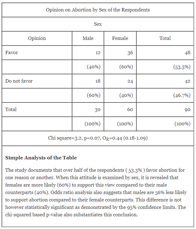
As an example, imagine that we are analyzing a survey question that asks: Do you approve of abortion (Yes/No).
We find from a preliminary analysis that gender is an important variable in determining response to this question and decide to construct a bivariate table containing these two variables.
A person’s opinion cannot affect his/her sex, but sex can affect opinion. Thus sex is the independent variable, and opinion on abortion is the dependent variable.
The table below shows the results of this investigation.
By percentage of the independent variable (sex), we can see whether a change in the independent variable (e.g., from male to female) results in a different distribution of yes/no (i.e., favor/do not favor) score on the dependent variable.
Here is a possible analysis of the table;
The types of analytical techniques that are appropriate for studying bivariate relationships depend on the nature of the variables-whether they are nominal, ordinal, or interval.
We present below a brief overview of the type of data needed to accomplish different types of bivariate analyses indicating the possible statistical test that can be applied.
When the data are measured on a nominal scale
Most often, we are interested in determining whether the observed differences within the data could have occurred by chance alone. In the example above, where both the variables are nominal, 40% of the males in contrast to 60% of the females are in favor of abortion.
Is this difference statistically significant, or could it have happened by chance alone? Probably, the most commonly used statistical test is the chi-square test to answer the question.
However, the chi-square statistic does not measure the strength of the relationship.
For this purpose, a “measure of association” is needed. For this purpose, we can employ such measures as phi-coefficient and Cramer’s V, which are derived from chi-square value.
When the data are measured on the ordinal scale
There are several different measures of association for cross-tabulations of ordinally measured variables.
Perhaps the most commonly used measure of association for such tables is called Gamma. The fourfold form of gamma is called Yule’s Q.
When the table has more than four cells, the Q coefficient is called gamma instead of Q. The chief disadvantage of gamma as a measure of association is that there is no simple significance teat for evaluating gamma.
When the data are measured on an interval scale
Relationships between interval variables may be studied with or without cross-tabulation.
If crosstabulation is made of interval variables, one can attempt computing gamma or Cramer’s V, examining the apparent nature of the relationship between the variables.
It is, however, more common to measure the relationship between pairs of interval variables without reference to any crosstabulations using Pearson’s product-moment correlation coefficient denoted by r. A t-test can assess the statistical significance of r.
The correlation coefficient tells us how strongly two variables measured on at least an interval scale are related. Still, it does not enable us to predict an individual’s value or score on one variable from knowledge of his or her score on the second variable.
Regression analysis is a technique that allows us to make such a prediction.
In this case, the measure of association is the zero-order regression coefficient, which indicates the average amount of change in the dependent variable associated with a unit change in the independent variable.
Here too, we have scope for testing the significance of the regression coefficient statistically.
Tri-variate Analysis
The recognition of a meaningful relationship between variables generally signals a need for further investigation. Even if one finds a statistically significant relationship, the question of why and under what conditions remain.
The introduction of a third variable called the control variable to interpret the relationship is often necessary.
Cross tabulations of three variables serve as the framework for such analysis. The most common three-variable table is the 2x2x2 table containing 3 dichotomous variables.
Look back to the 2×2 table describing the opinion of 90 respondents by sex. We can extend this 2×2 table to a 2x2x2 table simply by adding another variable, say religion, which is believed to affect the relationship between gender and attitude on abortion.
That is, the effect of gender on abortion attitude may be different for Muslims than for non-Muslim.
The resulting table will now look like as follows:

In this instance, religion is called a ‘control’ variable. The previous table showed the relationship between gender and abortion attitude, where religion was not known.
If we feel that the relationship between gender and attitude will be the same regardless of person’s religion, then there is no need to construct table 2, since both parts of table 2 will then yield identical results.
If, however, we feel that race will affect the relationship between gender and attitude, then we are predicting that interior cell frequencies in two halves of table 2 will be different.
That is a * e, b, and so on.
This effect, in which the relationship between two variables is dependent upon the third variable, is called statistical interaction effect’.
If we feel that religion will have such an effect, then the relationship shown in table 1 is inadequate and misleading and needs to be computed controlling for religion.
We say that race is controlled for because, within each cell of table 2, religion is constant (all Muslims or all non-Muslims) and thus cannot affect the result.
Multivariate Analysis
Analyses that permit a researcher to study the effect of controlling for one or more variables are called multivariate analyses since they involve multiple (more than two) variables.
Most multivariate techniques also permit the measurement of the degree of relationship between a dependent variable and two or more independent variables considered simultaneously.
The most commonly used multivariate techniques include, among others, are multiple regression analysis, multiple classification analysis (MCA), discriminating analysis, multivariate analysis of variance (MANOVA), logistic regression analysis, and hazard analysis.
Other methods in multivariate settings are factor analysis, cluster analysis, and multidimensional scaling. Multivariate techniques can be very powerful analytical tools, but they must be used with great caution.
They are all based on numerous assumptions that are very difficult to meet in most social science research. As a result, findings are not often valid.
Your plan of analysis should not include any multivariate techniques without being ensured of its applicability.
Before concluding this section, we emphasize here that as a first of multivariate analysis of data, the readers are advised to start with regression analysis.
What is the primary purpose of data analysis in research?
The primary purpose of data analysis in research is to test hypotheses, answer research questions, and further the overall goal of understanding social phenomena.
What is univariate analysis, and how is it used?
Univariate analysis refers to the examination of each variable separately. It involves transforming raw data into a form that makes it easy to understand and interpret, often by forming frequency distributions of single variables.
How does bivariate analysis differ from univariate analysis?
Bivariate analysis examines the relationship between two variables simultaneously, whereas univariate analysis looks at one variable at a time. Bivariate analysis can be used to study the interrelationships between two variables in a single table.
What is the role of a control variable in tri-variate analysis?
A control variable is introduced in tri-variate analysis to interpret the relationship between two other variables. It helps determine if the relationship between the two main variables depends on the third variable, known as a statistical interaction effect.
What are some commonly used multivariate techniques in data analysis?
Commonly used multivariate techniques include multiple regression analysis, multiple classification analysis (MCA), discriminating analysis, multivariate analysis of variance (MANOVA), logistic regression analysis, and hazard analysis.
Why should multivariate techniques be used with caution?
Multivariate techniques should be used cautiously because they are based on numerous assumptions that are often difficult to meet in most social science research, making the findings potentially invalid.
What is the significance of percentages in data analysis?
Percentages simplify data by reducing all numbers to a range from 0 to 100. They also translate the data into a standard form for relative comparison, making it easier to interpret and compare different data sets.