A multiplier is a number that indicates the magnitude of a particular macroeconomic policy measure. In other words, the multiplier attempts to quantify the additional effects of a policy beyond those that are immediately measurable.
For example, a decrease in taxation will have more of an effect than just the value of the reduced taxes. It will lead to greater disposable income which might cause an increase in consumption, which in turn might increase employment in industries that enjoy greater demand and so on.
So the total effect of the implemented policy equals the effect of the policy measure, times the multiplier. This is true for most macroeconomic policy measures because the actual effect of the measure cannot be quantified by the effect of the measure itself.
An example of a Multiplier
Multiplication:
6X3 = 18 Factor Factor Product (or multiplier) (or multiplicand)
In economics, the multiplier is the ratio of the increment in income to the increment in investment.
That is, multiplier, K=AY/AI
Calculating the value of the multiplier

Consumption Function
As the demand for a good depends upon its price, similarly consumption of a community depends upon the level of income. In other words, consumption is a function of income. The consumption function relates the amount of consumption to the level of income. When the income of a community rises, consumption also rises.
How much consumption rises in response to a given increase in income depends upon the marginal propensity to consume. It should be borne in mind that the consumption function is the whole schedule that describes the amounts of consumption at various levels of income.
The consumption function, or Keynesian consumption function, is an economic formula representing the functional relationship between total consumption and gross national income. It was introduced by British economist John Maynard Keynes, who argued the function could be used to track and predict total aggregate consumption expenditures.
The consumption function is represented as:
C = a + bY Where: C = Consumer spending a = Autonomous consumption b = Marginal propensity to consume Y = Real disposable income
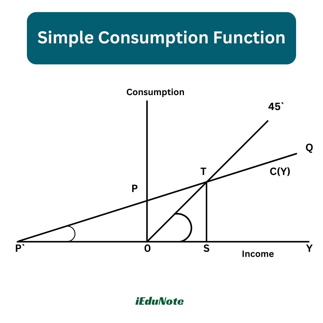
The consumption function, PQ, is a straight line and OT is a straight line passing through the origin making an angle of 45° which intersects the consumption function from below at point T.
This consumption function PQ satisfies all the following four characteristics.
According to Keynes, the consumption function must have the following characteristics:
- 1. Aggregate real consumption expenditure is a stable function of real income.
- 2. The marginal propensity to consume (MPC) or the slope of the consumption function defined as DC/dY must lie between zero and one i.e. 0 < MPC < 1.
- 3. The average propensity to consume (APC) or the proportion of income spent on consumption defined as C/Y should decrease as income increases.
- From the relation between marginal and average, we know that when the average falls, marginal is below average.
- Thus, when the average propensity to consume (APC) falls, the marginal propensity to consume (MPC) must be lower than the APC.
- 4. The marginal propensity to consume (MPC) itself probably decreases or remains constant as income increases.
Average propensity to consume
The average propensity to consume (APC) expresses the percentage of income consumed at any given level of income. In other words, it’s the amount of income the average consumer spends on goods and services.
The basic assumptions are
- (1) Price level stability
- (2) Self-sufficient economy
- (3) No undistributed profits
- (4) No state sector
The total consumption depends on the total income and there is a positive correlation between the two.
The average propensity to consume formula is calculated by dividing total consumption (what is spent on goods and services) by total income (what is earned) in a given period.
Therefore, the equation for APC is: Average propensity to consume (APC) = Total Consumption Expenditure / Total Disposable Income = C/Y
Marginal propensity to consume
In economics, the marginal propensity to consume (MPC) is an empirical metric that quantifies induced consumption, the concept that the increase in personal consumer spending (consumption) occurs with an increase in disposable income (income after taxes and transfers).
The proportion of the disposable income that individuals desire to spend on consumption is known as the propensity to consume. MPC is the proportion of additional income that an individual desires to consume.
For example, if a household earns one extra Dollar of disposable income, and the marginal propensity to consume is 0.65, then of that Dollar, the household will spend 65 poisa and save 35 poisa.
Mathematically, the MPC function is expressed as the derivative of the consumption function C concerning disposable income Y.
MPC = dC/dY
Or
MPC = ΔC / ΔY
Where ΔC is the change in consumption, and ΔY is the change in disposable income that produced the consumption.
Marginal propensity to consume can be found by dividing the change in consumption by a change in income, or, MPC = ΔC/ΔY. The MPC can be explained with a simple example
Here ΔC = 50, ΔY = 60, Therefore, MPC = ΔC/ΔY = 50/60 = 0.83 or 83%.
For example, you receive a bonus with your paycheck, and it is $500 on top of your annual earnings. You suddenly have $500 more in income than you did before.
If you decide to spend $400 of this marginal increase in income on a business suit, your marginal propensity to consume will be 0.8 ($400/ $500)
MPC and the Multiplier
Writing the equation for the equilibrium level of income, we have Y = C + I. Therefore, ΔY = ΔC + ΔI.
From the consumption function we know, C = a + bY. That is, ΔC = bΔY.
Now substituting this value in the above equation, we get ΔY = bΔY + ΔI.
ΔY – bΔY = ΔI.
ΔY(1 – b) = ΔI.
ΔY = (1 / (1 – b)) * ΔI.
ΔY / ΔI = 1 / (1 – b).
Therefore, multiplier K = ΔY / ΔI = 1 / (1 – MPC) = 1 / MPS.
Importance of Multiplier

The limitations and the criticism discussed here do have validity. However, none can undermine the importance of the investment multiplier in economic analysis. Based on the multiplier, Keynes advocated investment in public works during the depression.
The government as well as the private entrepreneurs can significantly expand the economic activities through the investment.
This investment will have an amplified effect on the income, output, and employment of the economy.
The multiplier is an important part of Keynes’s theory of income and employment. The concept of the multiplier is of great significance in economic analysis and policy.
Saving Investment Equality
The multiplier theory highlights the importance of investment in the theory of income and employment. As the consumption function is stable during the short run, fluctuations in income and employment are the result of fluctuations in the level of investment.
A rise in investment causes a cumulative rise in income and employment through the multiplier process and vice-versa.
The multiplier theory not only explains the process of income propagation as a result of a rise in the level of investment, but it also helps in bringing equality between saving and investment.
In case of divergence between the two, a change in the level of investment leading to a change in the level of income via the multiplier process, ultimately equalizes saving and investment.
Business Cycles
The multiplier process explains and helps in controlling different phases of business cycles occurring due to fluctuations in the level of income and employment.
The boom period (high level of income and employment) can be controlled by a reduction in investment, which leads to a cumulative decline in income and employment in the multiplier process.
On the other hand, during the depression phase of the business cycle (low level of income and employment), an increase in investment leads to a revival. If this process continues, then depression may turn into a boom period.
Formulation of Economic Policies
The government can decide upon the amount of investment to be injected into the economy to reduce unemployment. The multiplier theory helps the government in formulating an appropriate employment policy during the depression.
During the depression, the Government’s public works programs are more effective than the cheap money policy due to the multiplier effect of investment. It is important to note that any increase in investment in one sector should not be practiced.
Uses of Multiplier

- 1. The multiplier principle occupies a very important place not only in economic theory but also in shaping economic policy.
- 2. It plays a vital role as an instrument of income building.
- 3. It tells us how a small increase in investment can result in a large increase in aggregate income.
- 4. Multiplier uses control of business cycles.
- 5. It furnishes guidelines for appropriate income and employment policies.
- 6. It also explains the expansion of the public sector in modern times.
Limitations of Multiplier
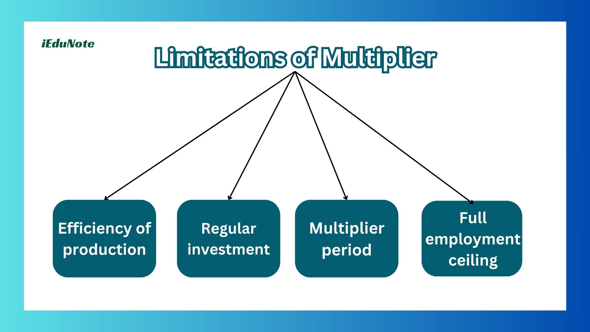
Efficiency of production
If the production system of the country cannot cope with the increased demand for consumption goods and make them readily available, the income generated will not be spent as visualized. As a result, the MPC may decline.
Regular investment
The value of the multiplier will also depend on regularly repeated investments.
Multiplier period
Successive doses of investment must be injected at suitable intervals if the multiplier effect is not being lost.
Full employment ceiling
As soon as full employment of the idle resources is achieved, further beneficial effects of the multiplier will practically cease.
Illustration 1:
In an economy, the basic equations are as follows: the consumption function is C = 300 + 0.8Y and the planned investment is I = $360 million. You are required to ascertain the following:
- The equilibrium level of income
- The equilibrium level of income when planned investment increases from 360 to 400 million, a total increase of 40 million
- The multiplier effect of the 40 million increases in planned investment.
Solution:
- The equilibrium condition is given as Y = C + I: Y = 300 + 0.8Y + 360 Y – 0.8Y = 300 + 360 0.2Y = 660 Y = 3,300
The equilibrium level of income is Y = $3,300 million.
- The equilibrium condition is given as Y = C + I: Y = 300 + 0.8Y + 400 Y – 0.8Y = 300 + 400 0.2Y = 700 Y = 700 / 0.2 Y = 3,500
Hence, the equilibrium level of income is $3,500 million.
- The equilibrium level of income increases from 3,300 to 3,500 crores when planned investment increases from 360 to 400 million. There is an increase in income by 200 million. Hence the multiplier effect is m = 1 / (1 – 0.8) = 5.
Illustration 2:
Presume in an economy the marginal propensity to consume is 0.75 and the level of autonomous investment decreases by 40 million. Find the following:
- The change in the equilibrium level of income
- The change in consumption expenditures
Solution:
The change in income is given by AY = m * AI, where m is the investment multiplier. Also, m = 1 / (1 – b), where b is the marginal propensity to consume.
Wc know ^Y / ^I = m
Therefore, the decrease in autonomous investment causes a decrease in the equilibrium level of income by 160 million.
Y = C + I, Therefore, AY = AC – 40 AC = -120
The consumption expenditure decreases by 120 million.
Illustration 3:
Compute the value of the investment multiplier when the marginal propensity to consume is (1) 0.80, (2) 0.65, (3) 0.40, and (4) 0.25. Find the effect of a decrease in the equilibrium income when autonomous investment decreases by 60 million when the marginal propensity to consume is (1) 0.80, (2) 0.65, (3) 0.40, and (4) 0.25.
Solution:
The value of m, the investment multiplier is: m = 1 / (1 – b)
Therefore: (1) m = 1 / (1 – 0.80) = 1 / 0.20 = 5 (2) m = 1 / (1 – 0.65) = 1 / 0.35 = 2.87 (3) m = 1 / (1 – 0.40) = 1 / 0.60 = 1.67 (4) m = 1 / (1 – 0.25) = 1 / 0.75 = 1.33
Thus, the decrease in the equilibrium income when autonomous investment decreases by 60 million is: (1) AY = AI * m = -60 * 5 = -300 (2) AY = AI * m = -60 * 2.87 = -172.2 (3) AY = AI * m = -60 * 1.67 = -100.2 (4) AY = AI * m = -60 * 1.33 = -79.8
Illustration 4:
In an economy, the marginal propensity to consume is 0.50. The level of autonomous investment decreases by 60 million. Find the following:
- The change in the equilibrium level of income
- The change in autonomous demand
- The induced change in the consumption expenditure
Solution:
- AY = m * AI, where m is the investment multiplier. Also, m = 1 / (1 – b), where b is the marginal propensity to consume.
AY = AI * m = -60 * 1 / (1 – 0.50) = -60 * 2 = -120
The decrease in autonomous investment causes a decrease in the equilibrium level of income by 120 million.
- The decrease in investment by 60 million is the change in the level of autonomous demand.
- Y = C + I, Therefore, AY = AC – 60 AC = -60
The consumption expenditure falls by 60 million.
Illustration 5:
Presume that in a two-sector economy, the income is $1000 million while the marginal propensity to consume is 0.40. Suppose the government wants to increase the income to $1600 million, by an amount of $600 million.
By how much should the autonomous investment be increased?
Solution:
The income level = $1000 million The planned income level is $1600 million Change in income = ΔY = 1600 – 1000 = $600 million
Thus the autonomous investment should be increased by $360 million for the income to increase to $1600 million. An increase in income by $600 million.